Using Twitter Sentiment Analysis to Predict Stock Price Movements of Major Companies via Support Vector Machines

Authors: Chris Charo, Hunter Clayton, and Camille Esteves

Introduction
Methods
Analysis & Results
Conclusion
References
Glossary

1. Introduction

1.1 Overview of Sentiment Analysis

Sentiment analysis is the process of analyzing text to derive the underlying emotions being expressed in a collection of data. It has a wide range of applications, including understanding customer satisfaction metrics, brand reputation, and marketing campaign responses. One area of sentiment analysis that has received significant attention is its relationship with public sentiment and the valuation of publicly traded companies and broader stock market indexes. With the S&P 500 Index currently boasting an aggregate market capitalization of $57.4 trillion, an advantage in predicting the price movements of publicly traded stocks would be highly valuable for investors (S&P Dow Jones Indices 2025). One of the most popular outlets for real-time public sentiment is the social media platform Twitter(X), which has over 586 million active users in 2025 (Statista 2025). Twitter(X) differentiates itself from other platforms through short-form content of 280 characters or fewer, allowing rapid communication of opinions, news, and humor (Chaires 2024). This concise format provides a valuable source of global sentiment data across generations, cultures, and regions. A multitude of tools are available for sentiment analysis, but Valence Aware Dictionary and sEntiment Reasoner (VADER), Financial Valence Aware Dictionary and sEntiment Reasoner (finVADER), and Financial Bidirectional Encoder Representations from Transformers (finBERT) excel at analyzing short-form content, making them an ideal choice for Twitter sentiment analysis.

1.2 Importance of Twitter Data in Financial Forecasting

Every day, millions of users share their perspectives on nearly every conceivable topic, including brands and companies. This constant flow of opinionated data makes Twitter(X) an invaluable resource for analyzing trends in public sentiment. In financial markets, these sentiments can serve as indicators of investor confidence, public reaction to corporate events, and potential short-term price fluctuations. Prior studies demonstrate that analyzing sentiment from Twitter posts can effectively reflect investor sentiment and broader market trends (Twitter Sentiment Analysis and Bitcoin Price Forecasting 2023).

1.3 Paper Roadmap

The remainder of this paper outlines the methodology for data preprocessing and model training, results of the sentiment and stock prediction analyses, and a discussion of findings with implications for financial forecasting. Overall, this study builds upon a growing body of literature that connects natural language processing, financial analytics, and social media data to improve predictive modeling in stock performance forecasting.

2. Methods

2.1 Sentiment Analysis

VADER

VADER is a popular lexicon-based sentiment analysis tool created by C.J. Hutto and Eric Gilbert at the Georgia Institute of Technology. Developed in 2014, VADER was designed specifically as a sentiment analysis tool that excelled at analyzing social media or “micro-blog like text”. VADER maintains a massive library of common words and phrases and functions by assigning a valence and intensity level score to each word in a block of text and aggregating those scores to determine an overall sentiment into one of three classes: positive, neutral, or negative.VADER is particularly advantageous for sentiment analysis because it delivers strong accuracy without requiring training data and operates extremely quickly (Hutto & Gilbert, 2014).

Code


vader = SentimentIntensityAnalyzer()

def vader_sentiment(text):
  scores = vader.polarity_scores(text)
  compound = scores['compound']

  if compound >= 0.05:
    return 'positive'
  elif compound <= -0.05:
    return 'negative'
  else:
    return 'neutral'

finished_dataset['vader_sentiment'] = finished_dataset['body'].apply(vader_sentiment)

print("Some samples from the Tweets:")
for i in range(5):
  print(f"{i+1}, {finished_dataset['body'].iloc[i]}\n")
print("\nSentiment distribution:")
print(finished_dataset['vader_sentiment'].value_counts())

finVADER

FinVADER is an open-source adaptation of the original VADER model, developed by Petr Koráb in 2023. It extends VADER’s lexicon-based approach by incorporating financial domain-specific lexicons, such as SentiBignomics and Henry’s Finance Lexicon, enabling more accurate sentiment analysis on financial texts like earnings reports, news articles, and finance specific tweets. Like VADER, FinVADER assigns valence and intensity scores to words and aggregates them to determine overall sentiment. By integrating domain-specific vocabulary, FinVADER improves the model’s ability to detect subtle positive or negative cues that are unique to financial language, while retaining VADER’s advantages of speed and not requiring training data to operate (Koráb, 2023).

Code


from tqdm import tqdm
tqdm.pandas()

def get_finvader_sentiment(text):
  scores = finvader(text, use_sentibignomics=True, use_henry=True, indicator='compound')

  if scores >= 0.05:
    return 'positive'
  elif scores <= -0.05:
    return 'negative'
  else:
    return 'neutral'

finished_dataset['sentiment_finVADER'] = finished_dataset['body'].progress_apply(get_finvader_sentiment)

finBERT

Bidirectional Encoder Representations from Transformers (BERT) is a deep learning language model developed by researchers at Google in 2018. BERT represented a major breakthrough in Natural Language Processing by introducing deep bidirectional training of transformer encoders. Prior to BERT, most NLP models processed text in a single direction (left-to-right or right-to-left), which limited their ability to capture full context and understand the relationships between words across a sentence. BERT’s bidirectional self-attention mechanism allows it to consider both preceding and following context simultaneously, resulting in much deeper language understanding. It has been widely adopted for tasks such as question answering, search query ranking, next-sentence prediction, text classification, and sentiment analysis (Devlin et al., 2019).

Similar to finVADER, finBERT is an open-source, domain-specific adaptation of the original BERT model. Introduced by Dogu Tan Araci in 2019, finBERT retains BERT’s underlying transformer architecture but is further pre-trained and fine-tuned on financial texts such as analyst reports, company announcements, and financial news. This domain adaptation enables the model to better capture financial terminology, linguistic patterns, and subtle sentiment cues, resulting in improved performance for financial sentiment classification tasks (Araci, 2019).

Code


from tqdm import tqdm

sentiments = []
batch_size = 4096

for i in tqdm(range(0, len(finished_dataset), batch_size)):
  texts = finished_dataset.iloc[i:i+batch_size]['body'].tolist()

  inputs = tokenizer(texts,
                     add_special_tokens=True,
                     max_length=512,
                     truncation=True,
                     padding=True,
                     return_attention_mask=True,
                     return_tensors='pt').to(device)

  with torch.no_grad():
    outputs = model(**inputs)
    sentiment = torch.nn.functional.softmax(outputs.logits, dim=1)
    sentiment_labels = sentiment.argmax(dim=1).cpu().numpy()
    label_map = {0: 'positive', 1: 'negative', 2: 'neutral'}
    batch_sentiments = [label_map[label] for label in sentiment_labels]
    sentiments.extend(batch_sentiments)

finished_dataset['finbert_sentiment'] = sentiments

2.2 Support Vector Machines (SVM)

Support Vector Machines are a supervised learning method that performs well in high dimensional classification tasks. In financial research, SVM is often used to detect patterns in market movement because it creates a margin-based decision boundary that reduces overfitting and can represent non-linear relationships using kernel transformations. Prior studies have shown that SVM models frequently outperform baseline approaches in stock movement prediction, especially when sentiment signals or other derived indicators are included in the feature set (Chakraborty et al. 2017).

In our project, SVM is not used for classifying tweet sentiment. Instead, the model is applied to predict whether the next trading day will experience a positive or negative price movement. Our workflow focuses on merging sentiment outputs with historical pricing data, aligning timestamps, and preparing a supervised dataset where each row contains aggregated sentiment scores and market variables such as daily returns and volume. The SVM then learns a decision boundary that separates upward and downward price outcomes based on these combined features. The purpose of using SVM in this context is to evaluate whether sentiment derived from Twitter provides meaningful predictive value beyond standard market indicators. By observing how the SVM separates classes when sentiment features are included, we can assess whether social media signals contribute observable structure to short horizon price behavior.

The non-linear kernel SVM model classifies into positive or negative class using the following decision function:

\[f(x) = {sgn} \left( \sum_{i=1}^{m} y_i \alpha_i \, k(x, x_i) + b \right)\]

$x$: Input feature vector
$m$: Number of support vectors
$y_i$: Label of the $i$-th support vector (+1 or -1)
$k(x, x_i)$: Kernel function
$b$: Bias term
$sgn$: Sign function, outputs +1 or -1 classification

Figure 1. Non-linear kernel SVM decision function (Schölkopf et al. 2002).

2.3 Model Implementation in this Study

The inputs used for the SVM model come from two main sources. First, we generated sentiment scores for each tweet using a combination of lexicon-based and transformer-based methods. These sentiment values were aggregated by date to match the daily resolution of the pricing data. Second, daily market features were added, including closing price change, opening price, high, low, and volume.

After merging the sentiment and pricing data, we constructed a supervised dataset where the target variable represents whether the next day’s closing price increased or decreased. SVM was chosen as one of the classification models in order to test whether sentiment features improve the separation of these two classes. The rbf kernel was selected for its efficiency and strong performance on structured financial datasets. The performance of the final model will allow us to compare how well sentiment-driven features contribute to forecasting compared to models that rely only on numerical market indicators.

2.4 Evaluation Metrics

We will evaluate the performance of the SVM model using a variety of methods: accuracy, precision, recall, and F-1 score. Accuracy score is the percentage of true positives and true negatives correctly identified by the model. Of all the predictions the model made, how many were correct?

\[\text{Accuracy Score} = \frac{\text{True Positives} + \text{True Negatives}}{\text{Total Predictions}}\]

Figure 2. Accuracy Score formula

While accuracy is an important metric, additional methods will be required to understand the model’s true ability to make predictions on stock price movements: Precision, Recall, and F-1 Score. The results of each metric will then be averaged and weighted to provide an overall evaluation.

Precision score measures the model’s ability to correctly identify true positives. Of all the cases the model predicted as positive, how many were actually positive?

\[\text{Precision} = \frac{\text{True Positives}}{\text{True Positives} + \text{False Positives}}\]

Figure 3. Precision formula

Recall measures the model’s ability to correctly identify the positive class, calculated as the proportion of actual positive cases that are correctly predicted as positive. Of all the actual positive cases, how many did the model correctly detect?

\[\text{Recall} = \frac{\text{True Positives}}{\text{True Positives} + \text{False Negatives}}\]

Figure 4. Recall formula

F-1 Score measures the balance between precision and recall. How well does the model balance precision and recall into a single score?

\[\text{F1} = \frac{2 \cdot \text{Precision} \cdot \text{Recall}}{\text{Precision} + \text{Recall}}\]

Figure 5. F1 Score formula

3. Analysis & Results

3.1 Overview of Datasets

This study utilizes two primary datasets to investigate the relationship between social media sentiment and stock market performance. The dataset used for sentiment analysis is titled ‘Tweets about the Top Companies from 2015 to 2020,’ created by Doğan, Metin, Tek, Yumuşak, and Öztoprak for the IEEE International Conference (Doğan et al. 2020). This dataset comprises over three million tweets collected using a Selenium-based parsing script designed to collect text data from Twitter(X). Each record includes tweet text, timestamp, company reference, and engagement attributes such as likes and retweets. The dataset serves as the foundation for sentiment analysis, enabling the classification of public opinion related to major NASDAQ companies.

Once sentiment classification is complete, the results will be used to predict the stock price movements of the companies included in the dataset. The stock data comes from ‘Values of Top NASDAQ Companies from 2010 to 2020,’ sourced directly from the NASDAQ website and hosted on Kaggle (Doğan et al. 2020). It includes daily historical stock prices: opening, closing, high, low, and volume data. To ensure analytical consistency, both datasets were merged based on overlapping date ranges. The merged dataset was further refined by removing extraneous or non-essential columns such as usernames, retweet indicators, and reply metadata. Before integration, data types were standardized, and timestamps were aligned to maintain temporal accuracy between social sentiment and corresponding stock data.

3.2 Data Preprocessing

Preprocessing is a critical step in preparing unstructured text data for machine learning applications, especially when working with social media content that is often noisy, informal, and contextually ambiguous (A Scoping Review of Preprocessing Methods 2023). The preprocessing phase for this project focused primarily on the textual component of the Twitter(X) dataset. Each tweet underwent a structured series of cleaning and transformation steps. Specifically, all text was first converted to lowercase to ensure consistency across the dataset. Subsequently, URLs, user mentions, hashtags, and stock symbols were removed, followed by tokenization based on whole words. Stop words were eliminated, with the exception of negation words such as ‘not’ and ‘no,’ which are critical in determining sentiment polarity. Lemmatization was then applied to reduce each word to its base form, allowing the models to better capture semantic meaning and context. Finally, the tweet body, a list of individually-separated words, are re-joined as a string (Du et al. 2024). These preprocessing methods align closely with those recommended in prior research emphasizing the importance of context retention and dimensionality reduction in text classification tasks (Financial Sentiment Analysis: Techniques and Applications 2024). Following these transformations, the finalized clean dataset was stored in a Pandas DataFrame, ready for sentiment classification.

Code


def lowercase_text(text):
  return text.lower()

finished_dataset['body'] = finished_dataset['body'].apply(lowercase_text)

def remove_noise(text):
  text = re.sub(r'http\S+|www\S+|https\S+', '', text, flags=re.MULTILINE)
  text = re.sub(r'@\w+', '', text)
  text = re.sub(r'\$[A-Z]+', '', text)
  text = re.sub(r'[^a-z\s]', '', text)
  text = ' '.join(text.split())
  return text

finished_dataset['body'] = finished_dataset['body'].apply(remove_noise)

def tokenize_text(text):
  tokens = word_tokenize(text)
  return tokens

finished_dataset['body'] = finished_dataset['body'].apply(tokenize_text)

stop_words = set(stopwords.words('english'))

negation_words = {'no', 'not', 'never', 'neither', 'nobody', 'nothing', 'nowhere', "n't"}
stop_words = stop_words - negation_words

def remove_stopwords(tokens):
  filtered_tokens = [word for word in tokens if word not in stop_words and len(word) > 2]
  return filtered_tokens

finished_dataset['body'] = finished_dataset['body'].apply(remove_stopwords)

import nltk
from nltk.stem import WordNetLemmatizer
nltk.download('wordnet')
lemmatizer = WordNetLemmatizer()

def lemmatize_tokens(tokens):
  lemmatized = [lemmatizer.lemmatize(word) for word in tokens]
  return lemmatized

finished_dataset['body'] = finished_dataset['body'].apply(lemmatize_tokens)

finished_dataset['body'] = finished_dataset['body'].apply(lambda x: ' '.join(x))

3.3 Dataset Visualizations

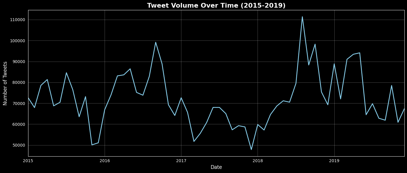
Tweet Volume Over Time

Code


plt.figure(figsize=(14, 6))
finished_dataset['date'] = pd.to_datetime(finished_dataset['date'])
tweets_per_month = finished_dataset.groupby(finished_dataset['date'].dt.to_period('M')).size()
tweets_per_month.plot(kind='line', color='skyblue', linewidth=2)
plt.title('Tweet Volume Over Time (2015-2019)', fontsize=16, fontweight='bold')
plt.xlabel('Date', fontsize=12)
plt.ylabel('Number of Tweets', fontsize=12)
plt.grid(alpha=0.3)
plt.tight_layout()
plt.show()

Tweet Volume Over Time

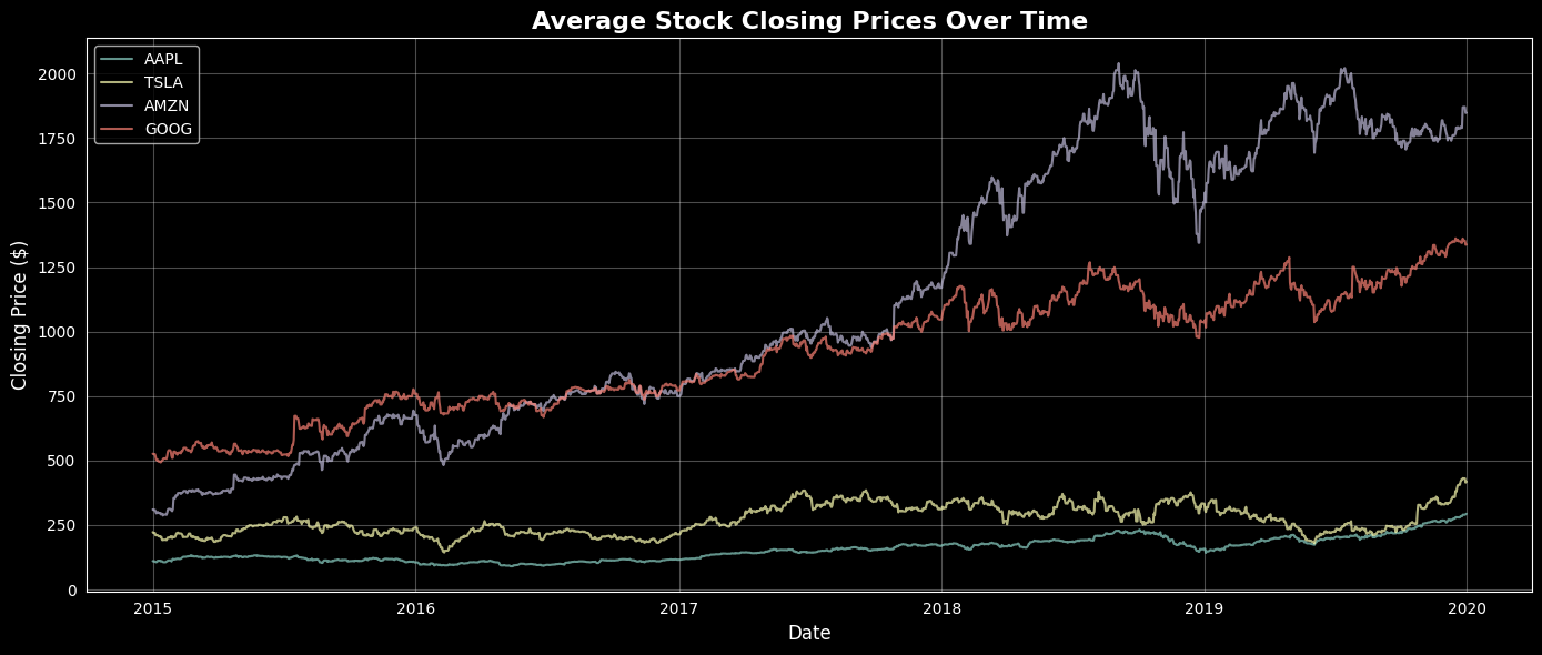
Average Stock Closing Prices Over Time

Code


plt.figure(figsize=(14, 6))
top_companies = finished_dataset['ticker_symbol'].value_counts().head(4).index # Top four to match the last visualization
for company in top_companies:
    company_data = finished_dataset[finished_dataset['ticker_symbol'] == company]
    plt.plot(company_data.groupby('date')['close_value'].mean(), label=company, alpha=0.7)
plt.title('Average Stock Closing Prices Over Time', fontsize=16, fontweight='bold')
plt.xlabel('Date', fontsize=12)
plt.ylabel('Closing Price ($)', fontsize=12)
plt.legend()
plt.grid(alpha=0.3)
plt.tight_layout()
plt.show()

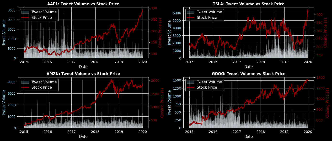
Average Stock Closing Prices Over Time

Average Stock Prices vs. Tweet Volume

Code


sns.set_style("dark")
plt.style.use("dark_background")

fig, axes = plt.subplots(2, 2, figsize=(14, 6))
axes = axes.flatten()

# Get top 4 companies by tweet volume
top_companies = finished_dataset['ticker_symbol'].value_counts().head(4).index

for idx, company in enumerate(top_companies):
    ax1 = axes[idx]

    # Filter the data for each company
    company_data = finished_dataset[finished_dataset['ticker_symbol'] == company].copy()

    # Group by date for tweet volume and average stock price
    daily_data = company_data.groupby('date').agg({
        'tweet_id': 'count',  # Count the tweets
        'close_value': 'mean'  # Average the closing price
    }).reset_index()

    # Create the dual axis since we are overlaying two graphs
    ax2 = ax1.twinx()

    # Plot tweet volume as bars
    ax1.bar(daily_data['date'], daily_data['tweet_id'], alpha=0.2, color='skyblue', label='Tweet Volume')
    ax1.set_ylabel('Tweet Volume', fontsize=11, color='skyblue')
    ax1.tick_params(axis='y', labelcolor='skyblue')

    # Plot stock price as line
    ax2.plot(daily_data['date'], daily_data['close_value'], color='darkred', linewidth=2, label='Stock Price')
    ax2.set_ylabel('Closing Price ($)', fontsize=11, color='darkred')
    ax2.tick_params(axis='y', labelcolor='darkred')

    # Formatting
    ax1.set_xlabel('Date', fontsize=11)
    ax1.set_title(f'{company}: Tweet Volume vs Stock Price', fontsize=11, fontweight='bold')
    ax1.grid(alpha=0.8)

    # Add legends
    lines1, labels1 = ax1.get_legend_handles_labels()
    lines2, labels2 = ax2.get_legend_handles_labels()
    ax1.legend(lines1 + lines2, labels1 + labels2, loc='upper left', fontsize=11)

plt.tight_layout()
plt.show()

Average Stock Prices vs. Tweet Volume

3.4 Sentiment Analysis Class Distributions

To evaluate the reliability of our automated sentiment classification methods, we created a manually labeled subset of 400 tweets. Three models were compared against these human-assigned labels: VADER, finVADER, and finBERT. Each method produced positive, neutral, or negative labels, which were aligned with the manual classifications to measure agreement.

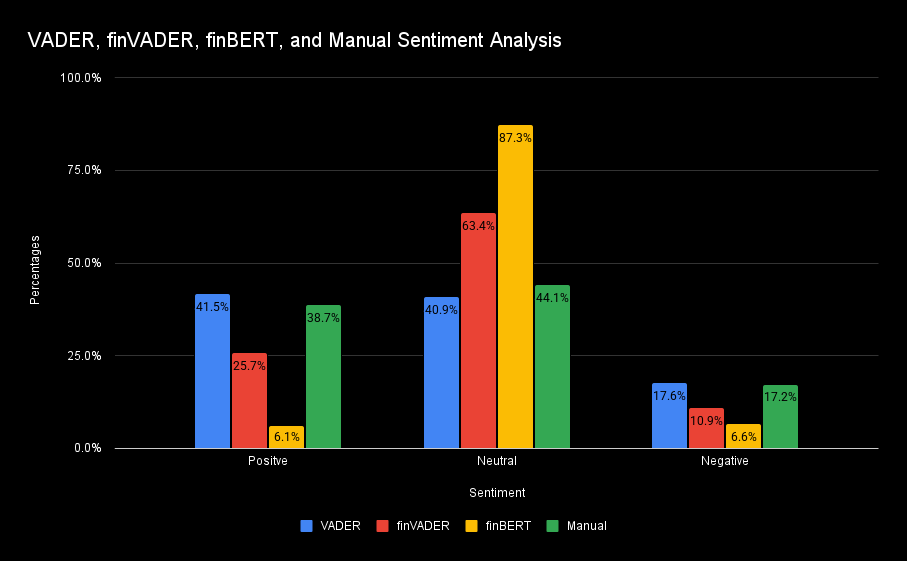
VADER, finVADER, finBERT, and Manual Sentiment Analysis Class Distribution Comparison

Figure 6. Sentiment Analysis Class Distribution of VADER, finVADER, finBERT, and Manual Sentiment Analysis

Across the 400-tweet evaluation set, VADER demonstrated the strongest alignment with human judgment, outperforming both finVADER and finBERT. This higher agreement supported its use as the primary labeling engine for the full dataset. Additionally, VADER offered two practical advantages: (1) faster runtime across the 4.3 million tweet corpus, and (2) consistent, interpretable scoring suitable for downstream aggregation.

Although finVADER and finBERT incorporate financial-domain specificity and transformer-based contextual understanding, they did not surpass VADER in agreement with human labels in our sample. Given the computational demands of these models and the scale of our dataset, the performance-to-cost tradeoff justified selecting VADER as our final sentiment classifier.

3.5 SVM Stock Market Prediction Results

After sentiment labeling was completed, the aggregated daily sentiment features were merged with daily stock price data to construct the supervised learning dataset. The Support Vector Machine (SVM) model was trained to classify next-day stock movement as either positive or negative. Performance was evaluated using accuracy, precision, recall, F1 score, ROC Curve, and confusion matrix analysis.

Code


import matplotlib.pyplot as plt
import seaborn as sns

plt.figure(figsize=(8, 6))
sns.heatmap(cm, annot=True, fmt="d", cmap="Blues", xticklabels=[0, 1, 2], yticklabels=[0, 1, 2])
plt.xlabel('Predicted')
plt.ylabel('True')
plt.title('Confusion Matrix')
plt.show()

Confusion Matrix

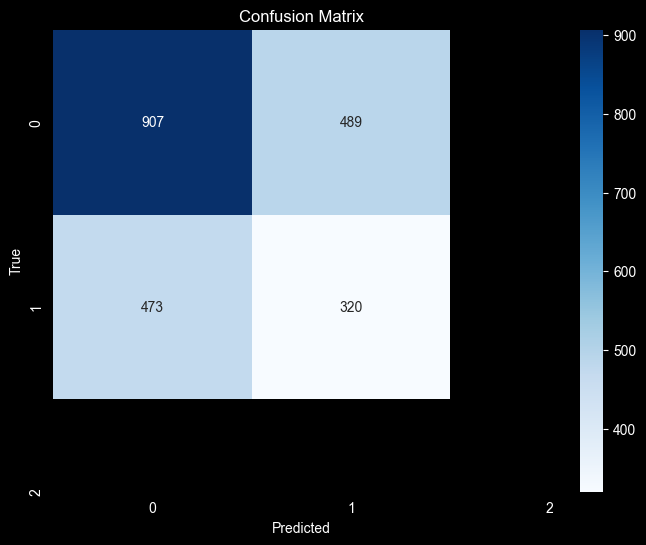
Figure 7. Confusion Matrix

This distribution indicates that the model correctly identified 907 negative-movement days and 320 positive-movement days, while misclassifying 489 false positives and 473 false negatives.

3.6 Evaluation Metrics

Code


from sklearn.metrics import accuracy_score, classification_report, confusion_matrix
final_model = SVC(kernel='rbf', C=best_C, gamma=best_gamma, class_weight='balanced')
final_model.fit(X_train_scaled, y_train)

y_pred = final_model.predict(X_test_scaled)
accuracy = accuracy_score(y_test, y_pred)

print("Final Model Results")
print(f"Test Accuracy: {accuracy*100:.2f}%)")
print("Confusion Matrix")
cm = confusion_matrix(y_test, y_pred)
print(cm)

Accuracy

\[\text{Accuracy Score} = \frac{\text{True Positives} + \text{True Negatives}}{\text{Total Predictions}}\] \[\text{Accuracy Score} = \frac{\text{320} + \text{907}}{\text{2,189}} ≈ {0.5607}\]

Precision

\[\text{Precision} = \frac{\text{True Positives}}{\text{True Positives} + \text{False Positives}}\] \[\text{Precision} = \frac{\text{320}}{\text{320} + \text{489}} ≈ {0.3950}\]

Recall

\[\text{Recall} = \frac{\text{True Positives}}{\text{True Positives} + \text{False Negatives}}\] \[\text{Recall} = \frac{\text{320}}{\text{320} + \text{473}} ≈ {0.4030}\]

F-1 Score

\[\text{F1} = \frac{2 \cdot \text{Precision} \cdot \text{Recall}}{\text{Precision} + \text{Recall}}\] \[\text{F1} = \frac{2 \cdot \text{0.3950} \cdot \text{0.4030}}{\text{0.3950} + \text{0.4030}} ≈ {0.3980}\]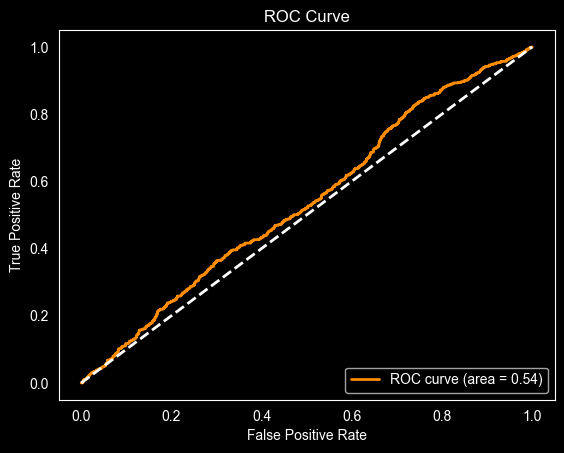

ROC Curve

Figure 8. ROC Curve

3.7 ROC Curve

The ROC curve provides a broader view of the SVM model’s predictive behavior by evaluating performance across all classification thresholds and summarizing the trade-off between the true positive rate and false positive rate. In financial prediction settings, sentiment signals may be noisy and influenced by external factors.

The model performs only slightly better than random chance, with an AUC of approximately 0.54, and the curve’s close alignment with the diagonal reference line suggests difficulty in differentiating stock price direction based solely on Twitter(X) sentiment.

Class imbalances, ambiguous sentiment, and linguistic variability reduce signal clarity, and prior work notes that context-aware models often outperform traditional classifiers. Overall, the ROC curve reinforces that sentiment alone is challenging for predicting next-day stock movement, and hybrid approaches combining financial indicators and sentiment are recommended (Financial Sentiment Analysis: Techniques and Applications 2024).

3.8 Interpretation

The SVM model demonstrated minimal predictive ability with an overall accuracy of 56.07 percent, which is above random chance for a binary classification task but still limited in practical predictive power. Incorporating sentiment features improved interpretability but produced only modest gains relative to expected market-based baselines.

A key observation from the confusion matrix is the model’s difficulty classifying both positive and negative movements with high precision. The false positive and false negative counts are relatively high, suggesting overlapping feature distributions between up-movement and down-movement classes. This may indicate that:

Sentiment signals from Twitter, while directionally informative, are noisy.
Daily aggregation may lose temporal nuance.
That next-day movement is influenced more strongly by market variables than by public sentiment alone.

Despite these limitations, the model highlights that sentiment features do contribute measurable predictive information, and their inclusion supports the broader hypothesis that public online discourse reflects market psychology.

3.9 Hyperparameter Tuning via Particle Swarm Optimization

Code


from sklearn.svm import SVC
from sklearn.model_selection import cross_val_score
!pip install pyswarm
from pyswarm import pso

def objective(params):
    C = params[0]
    gamma = params[1]

    svm = SVC(kernel='rbf', C=C, gamma=gamma, class_weight='balanced')
    scores = cross_val_score(svm, X_train_scaled, y_train, cv=5, scoring='f1_macro')

    return -scores.mean()

best_params, _ = pso(objective,
lb=[0.01, 0.0001],
ub=[100, 1.0],
swarmsize=15,
maxiter=20)

best_C = best_params[0]
best_gamma = best_params[1]

Prior to determining our final SVM model, we utilized Particle Swarm Optimization (PSO) To determine the optimal hyperparameters. PSO is a heuristic approach that mimics the behavior of swarming animals by combining their individual efforts across the entire swarm to maximize results.

An important step in setting up the PSO code is establishing the upper and lower bounds, which together define the search space. For an SVM using an RBF kernel, the C and Gamma parameters create a two-dimensional search space, with one parameter on the x-axis and the other on the y-axis. PSO uses individual elements, called particles, which act like independent animals within a group. A predefined number of particles are initialized and randomly placed within the search space. These particles then explore their local areas for the coordinates that yield the best result, under the assumption that a point with a good outcome will likely continue to improve in its immediate vicinity. The particles then communicate their findings to the swarm collectively. As a result, individual particles can begin moving toward the better results discovered by the group and, ideally, work together to identify the parameters that produce the “best” result.

The fact that particles are randomly scattered and will search somewhat independently is especially useful for avoiding local minima, whereas algorithms such as gradient descent may misidentify a local minimum as a global minimum. While PSO can incorporate additional parameters such as velocity and inertia, we used a more basic form that included only swarm size and maximum iterations (Tam, 2021)

While PSO was useful in our hyperparameter tuning experimentation, it did not significantly improve the model’s predictive performance. Although additional optimization methods could potentially yield further improvements, we believe the results, even after applying PSO, support our conclusion that Twitter sentiment alone is not sufficient to reliably predict future stock performance.

4. Conclusion

4.1 Limitations

While informative, only human-labeling a 400-tweet subset is a relatively small sample compared to the full dataset. While the subset offers a meaningful comparison, future research could expand the manually labeled set to strengthen the validation process and further benchmark model performance. For the SVM prediction model, Several constraints influenced the final performance:

The rbf kernel, chosen for efficiency with large datasets, may underfit complex patterns.
Sentiment was reduced to three categories, limiting granularity.
Merging at the daily level may obscure intraday sentiment–price relationships.

Future research could explore nonlinear kernels, ensemble models, or intraday sentiment features, as well as deeper fine-tuned transformer models for improved classification.

4.2 Concluding Remarks

The results show that the SVM model captures some relationship between Twitter sentiment and next-day stock movement, but the predictive strength remains moderate. Nevertheless, this analysis supports the idea that sentiment can supplement traditional market indicators and offers a foundation for more advanced predictive modeling in future analysis.

References

A Comparative Study of Sentiment Analysis on Customer Reviews Using Machine Learning and Deep Learning. 2023. Computers 13, no. 12 (340). https://www.mdpi.com/2073-431X/13/12/340 [Back to Top]

A Scoping Review of Pre Methods for Unstructured Text Data to Assess Data Quality. 2023. PLOS ONE. https://pmc.ncbi.nlm.nih.gov/articles/PMC10476151/ [Back to Top]

Chaires, Rita. 2024. “Ultimate Social Media Cheat Sheet: Character Limits & Best Days/Times to Post”. American Academy of Estate Planning Attorneys, February 6, 2024. https://www.aaepa.com/2022/05/ultimate-social-media-cheat-sheet-character-limits-best-days-times-to-post [Back to Top]

Chakraborty, P., U. S. Pria, M. R. A. H. Rony, and M. A. Majumdar. 2017. “Predicting Stock Movement Using Sentiment Analysis of Twitter Feed.” In Proceedings of the 2017 6th International Conference on Informatics, Electronics and Vision (ICIEV), 1–6. Himeji, Japan. https://doi.org/10.1109/ICIEV.2017.8338584 [Back to Top]

Doğan, M., Ö. Metin, E. Tek, S. Yumuşak, and K. Öztoprak. 2020. “Speculator and Influencer Evaluation in Stock Market by Using Social Media.” In Proceedings of the 2020 IEEE International Conference on Big Data (Big Data), 4559–4566. Atlanta, GA. https://doi.org/10.1109/BigData50022.2020.9378170 [Back to Top]

Du, Ke-Lin, Bingchun Jiang, Jiabin Lu, Jingyu Hua, and M. N. S. Swamy. 2024. “Exploring Kernel Machines and Support Vector Machines: Principles, Techniques, and Future Directions.” Mathematics 12, no. 24: 3935. https://doi.org/10.3390/math12243935 [Back to Top]

Financial Sentiment Analysis: Techniques and Applications. 2024. ACM Computing Surveys. https://dl.acm.org/doi/pdf/10.1145/3649451 [Back to Top]

Kolasani, Sai Vikram, and Rida Assaf. 2020. “Predicting Stock Movement Using Sentiment Analysis of Twitter Feed with Neural Networks.” *Journal of Data Analysis and Information * 8 (4): 309–319. https://doi.org/10.4236/jdaip.2020.84018 [Back to Top]

S&P Dow Jones Indices. 2025. “S&P 500®.” Accessed October 2, 2025. https://www.spglobal.com/spdji/en/indices/equity/sp-500/#overview [Back to Top]

Statista. 2025. “Most Used Social Networks 2025, by Number of Users.” March 26, 2025. https://www.statista.com/statistics/272014/global-social-networks-ranked-by-number-of-users [Back to Top]

Twitter Sentiment Analysis and Bitcoin Price Forecasting: Implications for Financial Risk Management. 2023. ProQuest. https://www.proquest.com/scholarly-journals/twitter-sentiment-analysis-bitcoin-price/docview/3047039752/se-2 [Back to Top]

Schölkopf, Bernhard, and Alexander J. Smola. Learning with Kernels: Support Vector Machines, Regularization, Optimization, and Beyond. Cambridge, MA: The MIT Press, 2002. Accessed December 5, 2025. https://mcube.lab.nycu.edu.tw/~cfung/docs/books/scholkopf2002learning_with_kernels.pdf . [Back to Top]

Chen, Tianqi, and Carlos Guestrin. “XGBoost: A Scalable Tree Boosting System.” In Proceedings of the 22nd ACM SIGKDD International Conference on Knowledge Discovery and Data Mining, 785–94. New York, NY, USA: ACM, 2016. https://doi.org/10.1145/2939672.2939785. [Back to Top]

Qin, Chuan, Liangming Chen, Zangtai Cai, Mei Liu, and Long Jin. 2023. “Long Short-Term Memory with Activation on Gradient.” Neural Networks 164: 135–145. https://doi.org/10.1016/j.neunet.2023.04.026. [Back to Top]

Nguyen, Anh & Nguyen, Phi Le & Vu, Viet & Pham, Quoc & Nguyen, Viet & Nguyen, Minh Hieu & Nguyen, Hùng & Nguyen, Kien. (2022). Accurate discharge and water level forecasting using ensemble learning with genetic algorithm and singular spectrum analysis-based denoising. Scientific Reports. 12. 10.1038/s41598-022-22057-8. [Back to Top]

Hutto, C, and Eric Gilbert. “VADER: A Parsimonious Rule-Based Model for Sentiment Analysis of Social Media Text.” Proceedings of the International AAAI Conference on Web and Social Media 8, no. 1 (2014): 216–25. https://doi.org/10.1609/icwsm.v8i1.14550. [Back to Top]

Koráb, Petr. FinVADER: VADER Sentiment Classifier Updated with Financial Lexicons. GitHub. Apache‑2.0. December 6, 2023. Accessed November 22, 2025. https://github.com/PetrKorab/FinVADER [Back to Top]

Jacob Devlin, Ming-Wei Chang, Kenton Lee, and Kristina Toutanova. 2019. “BERT: Pre-training of deep bidirectional transformers for language understanding.” Proceedings of the 2019 Conference of the North 2019:4171-. https://doi.org/10.18653/v1/n19-1423. [Back to Top]

Araci, Dogu. “FinBERT: Financial Sentiment Analysis with Pre-Trained Language Models,” 2019. https://doi.org/10.48550/arxiv.1908.10063. [Back to Top]

Tam, Adrian. “A Gentle Introduction to Particle Swarm Optimization.” MachineLearningMastery.com, October 12, 2021. https://machinelearningmastery.com/a-gentle-introduction-to-particle-swarm-optimization/. [Back to Top]

Glossary

Twitter(X) — In 2022, Twitter was acquired and rebranded as X. Although the dataset used in this report contains pre-acquisition data, we reference both names for clarity and to preserve the original meaning and context.

Tweets(Posts) — Post acquisition, Tweets were renamed to Posts on X.

SVM — Support Vector Machines

VADER — Valence Aware Dictionary and sEntiment Reasoner

finVADER — Financial Valence Aware Dictionary and sEntiment Reasoner

finBERT — Financial Bidirectional Encoder Representations from Transformers

NLP — Natural Language Processing

PSO — Particle Swarm Optimization

Back to Home

SVM Capstone Project

A project exploring stock market prediction with SVM and Twitter sentiment

Using Twitter Sentiment Analysis to Predict Stock Price Movements of Major Companies via Support Vector Machines

Table of Contents

1. Introduction

1.1 Overview of Sentiment Analysis

1.2 Importance of Twitter Data in Financial Forecasting

1.3 Paper Roadmap

2. Methods

2.1 Sentiment Analysis

VADER

finVADER

finBERT

2.2 Support Vector Machines (SVM)

2.3 Model Implementation in this Study

2.4 Evaluation Metrics

3. Analysis & Results

3.1 Overview of Datasets

3.2 Data Preprocessing

3.3 Dataset Visualizations

Tweet Volume Over Time

Average Stock Closing Prices Over Time

Average Stock Prices vs. Tweet Volume

3.4 Sentiment Analysis Class Distributions

3.5 SVM Stock Market Prediction Results

3.6 Evaluation Metrics

Accuracy

Precision

Recall

F-1 Score

3.7 ROC Curve

3.8 Interpretation

3.9 Hyperparameter Tuning via Particle Swarm Optimization

4. Conclusion

4.1 Limitations

4.2 Concluding Remarks

References

Glossary

Using Twitter Sentiment Analysis to Predict Stock Price Movements of Major Companies via Support Vector Machines

Table of Contents

1. Introduction

1.1 Overview of Sentiment Analysis

1.2 Importance of Twitter Data in Financial Forecasting

1.3 Paper Roadmap

View Detailed Literature Review & Related Work

2. Methods

2.1 Sentiment Analysis

VADER

finVADER

finBERT

2.2 Support Vector Machines (SVM)

2.3 Model Implementation in this Study

2.4 Evaluation Metrics

3. Analysis & Results

3.1 Overview of Datasets

3.2 Data Preprocessing

3.3 Dataset Visualizations

Tweet Volume Over Time

Average Stock Closing Prices Over Time

Average Stock Prices vs. Tweet Volume

3.4 Sentiment Analysis Class Distributions

3.5 SVM Stock Market Prediction Results

3.6 Evaluation Metrics

Accuracy

Precision

Recall

F-1 Score

3.7 ROC Curve

3.8 Interpretation

3.9 Hyperparameter Tuning via Particle Swarm Optimization

4. Conclusion

4.1 Limitations

4.2 Concluding Remarks

References

Glossary